SALMS R-package

Introduction

SALMS (Signal Analyses for Land Monitoring Systems) is an R package that can help with analayses of remote sensing signals. The text below is mainly taken from the vignette of the package. The package is currently in the CBM repository in GitHub: https://github.com/ec-jrc/cbm/tree/main/scripts/SALMS can be installed directly in R with the command:

install_github("ec-jrc/cbm/scripts/SALMS")

The background for this package is that land cover objects are commonly observed through remote sensing. The change in land cover leads to changes in the observed remote sensing signal for an area of interest. This area could be any spatially represented feature (i.e., an agricultural parcel, forest unit). Ideally, it should have a homogeneous cover, for which we will expect all parts to react similar to an activity, with normal statistical variability.

The package was developed for help with detection of agricultural activities (typically mowing, ploughing, harvesting etc.), but can also be used for other applications. An example could be help for detection of illegal activities in natural reserves. The functions are most efficient when the single activity takes place within the entire area or feature of interest (FOI), otherwise the response depends on the proportion of the land that was changed by the activity.

This package covers much of the functionality described in the report “Proposed workflow for optimization of land monitoring systems” by Zielinski et al. (2022). The following text is mainly copied from the abstract of the report.

The background of the report is that Member States in the European Union are responsible for implementing the payment schemes to farmers. Checks of farmer activity have traditionally been performed with on-the-spot-checks, but with the free access to wall-to-wall satellite imagery from the European Copernicus programme, Checks by Monitoring was introduced to reduce of the controls burden and facilitate the management of early warnings in combination with an option to correct the aid application that could prevent non-compliances. The automation of this process helped to move it from a sample-based approach to covering the full population.

Much work has already been done regarding cloud-based solutions and large-scale detection of activities, but less attention was given to understanding the relationship between the activity and the corresponding signals, and in general the signal behaviour. This report describes a framework that could be followed to analyse the signal behaviour from a large number of bands and indices from remote sensing sensors, and to select one or a few of them as potential candidates for marker development. In the analysed data sets, indices from Sentinel-2 appears to have better discriminative power than those from Sentinel-1, but also the latter can give good results for countries where clouds reduce the availability of Sentinel-2 images. Several different statistical descriptors of the remote sensing pixels appeared to give equally good results (P25, P50, P75 and mean), but because that the median is less affected by outliers, it would be the recommended choice.

The result of signal behaviour analyses highly depends on quality and level of details of input data and are based on ground truth data, the signal time series are computed from image pixels located inside the boundaries of a feature of interest (agricultural parcel) and dates of activities. The signal selection approach is generic and can be applied to any land monitoring system where there is an interest in changes on a preselected field. The method is adjustable, exploring (by providing a sequence of statistical methods) links between local knowledge and practices on the one side, and remote sending images and the derived signals on the other side.

Throughout this package, we will refer to these areas as a feature of interest, FOI. Instead of analysing all pixels within the FOI object, the functionality in this package is based on a reduction of the areal observations by different statistical descriptors for each signal source.

Descriptors

The most common statistical descriptors are the ones such as mean, quantiles, standard deviation. However, there are many more, including higher order moments (skewness and curtosis) or entropy. The default version uses 19 different descriptors, from the functions fivenum, stat.desc, and the entropy. If vec is the set of a signal values for the different pixels within a Feature of Interest (FOI), the descriptors would be:

# Example data for showing the descriptors
library(pastecs)
library(entropy)
vec = 1:10
fivenum(vec)
#> [1]  1.0  3.0  5.5  8.0 10.0
stat.desc(vec, basic = FALSE, norm = TRUE)
#>       median         mean      SE.mean CI.mean.0.95          var      std.dev
#>    5.5000000    5.5000000    0.9574271    2.1658506    9.1666667    3.0276504
#>     coef.var     skewness     skew.2SE     kurtosis     kurt.2SE   normtest.W
#>    0.5504819    0.0000000    0.0000000   -1.5616364   -0.5852118    0.9701646
#>   normtest.p
#>    0.8923673
entropy.empirical(vec)
#> [1] 2.151282

The package does not include the functionality for extracting these the time series from the remote sensing images.

Input data

The analyses start with two types of .csv-files:

• A file with the dates and types of the activities, the ground truth (in-situ data, observed on the ground)

• Several files with time series of remote sensing observations

The intention is to include more flexibility regarding names, but for the moment, the time series need to have names reflecting their content based sensor source i.e. Sentinel-1 and Sentinel-2.

FOIinfo

The ground truth are read into FOIinfo which is a data.frame. This should contain an overview of the activities and corresponding FOIs of interest. The columns with the following names are necessary (also lower case accepted):

• ID: The ID of the FOI (the function also accepts PSEUDO_ID or FIELD_ID

• EVENT_DATE: When did the activity happen (or start)? Also ACTIVITY_DATE or EVENT_START_DATE are accepted names

• EVENT_TYPE: This column should have a code for each type of activities that should be analysed

The package is quite flexible with date formats (mm-dd-yyyy, yyyy-mm-dd, etc), and will try to parse with different formats and see which one works.

The following shows the first 6 events of the example data set.

ddir = system.file("extdata", package = "SALMS")
FOIinfo = read.csv(paste0(ddir, "/gtdir/FOIinfo.csv"))
head(FOIinfo)
#>   X ID area Event_date Event_type
#> 1 0  1  1.3 10/07/2020          1
#> 2 1  2  0.9 13/06/2020          1
#> 3 2  3  0.8 01/07/2020          1
#> 4 3  4  1.3 27/06/2020          1
#> 5 4  5  1.2 25/07/2020          1
#> 6 5  6  1.3 30/06/2020          1

This example also includes the area (in ha in this case). One FOI can have several activities observed (i.e. throughout the season) .

ts-files

The .csv-files with time series should be stored in a single directory, for each area of interest and for each group of remote sensing signals/indexes These files should have names according to their content. The intention is to include more flexibility regarding names, but for the moment, the time series need to have names reflecting their content based on Sentinel-1 and Sentinel-2.

Five different file names are expected (where ID is the ID of the FOI, the same as the ID of the FOIinfo object above:

• ID_s1_coh6_ts.csv - The different time series for the coherence (including ratios between orbits)

• ID_s1_bs_ts.csv - The different time series for the back scatter (including ratios between orbits)

• ID_s2_ts.csv - The different time series for S2-bands

• ID_s2_idx_ts.csv - The different time series for different derived S2-indexes

• ID_s1_bsidx_ts.csv - The different time series for indexes derived from the backscatter

All these time series need some particular columns for the function createSignals to be able to create the activity centred time series:

• Date: the date (and time) of the acquisition. This date might be an average for example for s1_coherence signals that are averages of different orbits or different polarizations. Ideally, these data sets should already also include the week column, which identifies the week of the year of the observations

• Week: this column is optional, but should be available for data sets that already include weekly averaged signals, such as averages of different polarizations and orbits.

• Band: One file can include many different bands, and this column should include the band name for each observation.

• Orbit: This one is only relevant for S1-signals. It can be omitted if the orbit can be found from the date (if it also includes the time of the acquisition).

• Count: This is optional, and only necessary if the analyses should use a weighting factor (weighted = TRUE) in the analyses

• Descriptors: The remaining columns should have the time series for the different descriptors, with the name of each descriptor as column name.

• Histogram values: This is an optional value, mainly used for S2-observations. This indicates the number of pixels within each class of the classification mask, for example shown towards the bottom of https://sentinels.copernicus.eu/web/sentinel/technical-guides/sentinel-2-msi/level-2a/algorithm.

The first lines of this file can look like this (with an example from the package)

ddir = system.file("extdata", package = "SALMS")
dat = read.csv(paste0(ddir, "/tsdir/1_s2_idx_ts.csv"))
head(dat)
#>   cwithin chalf call       date band count          MIN         P25         P50
#> 1      97   129  162 2020-01-04 GARI    97 -0.003617167  0.02064336  0.03525393
#> 2      97   129  162 2020-01-04 NDVI    97  0.056822895  0.07085278  0.07647305
#> 3      97   129  162 2020-01-04  BSI    97 -0.137596417 -0.13050421 -0.12518195
#> 4      97   129  162 2020-01-09 GARI    97 -0.108171637 -0.01309887  0.03287543
#> 5      97   129  162 2020-01-09 NDVI    97 -0.027041357  0.02374670  0.03428296
#> 6      97   129  162 2020-01-09  BSI    97 -0.089059923 -0.06720757 -0.05393071
#>           P75           MAX      MEDIAN        MEAN      SE.MEAN CI.MEAN.0.95
#> 1  0.04863408  0.0674882385  0.03525393  0.03439160 0.0017027393  0.003379911
#> 2  0.08255319  0.0914504466  0.07647305  0.07634766 0.0007639961  0.001516520
#> 3 -0.11880331 -0.1102410376 -0.12518195 -0.12463916 0.0006962173  0.001381980
#> 4  0.06209981  0.1299435028  0.03287543  0.02446510 0.0054877141  0.010893026
#> 5  0.04962647  0.0731707317  0.03428296  0.03427784 0.0021900500  0.004347215
#> 6 -0.04062024  0.0001388696 -0.05393071 -0.05181195 0.0021638233  0.004295155
#>            VAR     STD.DEV    COEF.VAR    SKEWNESS    SKEW.2SE   KURTOSIS
#> 1 2.812341e-04 0.016770037  0.48762009  0.08456523  0.17259951 -0.8771574
#> 2 5.661794e-05 0.007524489  0.09855559 -0.24484214 -0.49972826 -0.8114368
#> 3 4.701770e-05 0.006856946 -0.05501438  0.04777411  0.09750801 -1.0238479
#> 4 2.921156e-03 0.054047715  2.20917624 -0.34100108 -0.69599078 -0.5627923
#> 5 4.652429e-04 0.021569491  0.62925474 -0.52477203 -1.07107139 -0.1101928
#> 6 4.541667e-04 0.021311188 -0.41131801  0.52590902  1.07339200 -0.4396198
#>     KURT.2SE NORMTEST.W  NORMTEST.P  ENTROPY hist.0 hist.1 hist.2 hist.3 hist.4
#> 1 -0.9036716  0.9744203 0.054855823 4.449000      0      0      0      0      0
#> 2 -0.8359644  0.9746543 0.057152028 4.569847      0      0      0      0      0
#> 3 -1.0547961  0.9719646 0.035732764 4.573210      0      0      0      0      0
#> 4 -0.5798040  0.9780403 0.103555426 5.516926      0      0      0      0      0
#> 5 -0.1135236  0.9719588 0.035697146 4.468723      0      0      0      0      0
#> 6 -0.4529084  0.9634395 0.008412672 4.472277      0      0      0      0      0
#>   hist.5 hist.6 hist.7 hist.8 hist.9 hist.10 hist.11
#> 1      0      0      0      0     97       0       0
#> 2      0      0      0      0     97       0       0
#> 3      0      0      0      0     97       0       0
#> 4      0      0      0      0     97       0       0
#> 5      0      0      0      0     97       0       0
#> 6      0      0      0      0     97       0       0

The first columns refers to the number of pixels that are within the outline of the FOI, depending on the approach for selecting pixels on the border (the example only uses pixels completely within the boundary, the number which is the also repeated under count).

plotTimeSeries

Before starting the analyses, it would be advisable to plot some of the original time series first, with the function plotTimeSeries. The function can typically print to two different devices (usually two pdfs), where the first will include a high number of plots and the second one fewer.

library(SALMS)
# Read data from package directory
ddir = system.file("extdata", package = "SALMS")
tsdir = paste0(ddir, "/tsdir")

# Output to tempdir, change to something local for easier access to pdfs
bdir = tempdir()

# File with activity information
FOIinfo = read.csv(paste0(ddir, "/gtdir/FOIinfo.csv"))

# Two output files
devs = list()
for (ipdf in 1:2) {pdf(paste0(bdir, "/ts_", ipdf, ".pdf")) ; devs[ipdf] = dev.cur()}

# Plot the individual signals to see their behaviour
plotTimeSeries(FOIinfo, devs = devs, tsdir = tsdir, plotAllStats = FALSE, iyear = 2020, legend = "before")
#> $s1_coh6
#> list()
#>
#> $s2
#> list()
#>
#> $s1_bs
#> list()
#>
#> $s2_idx
#> list()
#>
#> $s1_bsidx
#> list()
#>
#> $s1_coh6rat
#> list()
#>
#> $s1_bsrat
#> list()
for (ipdf in 1:2) dev.off(devs[ipdf])

# Plot of one of the individual time series
plotTimeSeries(FOIinfo[2,], obands = list(s2_idx = "NDVI"), stats = "P50", tsdir = tsdir, iyear = 2020)
#> $s2_idx
#> list()

Time series of signals for the 50th percentile of NDVI

Figure 1 above shows the time series for NDVI, for the P50 percentile. The black line shows the date of an activity (mowing of grass in this case), as indicated in the FOIinfo-file. For the NDVI, a drop in the signal value is observed after the activity took place.

The function can produce plots for all indexes and all descriptors, normally plotted in one or several pdfs. The legend is usually good for pdfs, less good in this example.

createSignals

The function createSignals will take the time series above and extract activity centred and weekly time series, with a length equal to 2*nweeks+1, meaning that the new time series will have the same number of weeks before and after the activity. The newly created time series will have the same columns as the time series in the input, but also a few extra, as it will include some of the information also from FOIinfo. Instead of being separate for each ID, they are separated for each signal, with the possibility of having data for all FOIs in the same file. The additional column names will be:

• EVENT_TYPE: This column is necessary if there is more than one activity type in the data set

• WEEK: The week number of the observation relative to the start of the activity centred time series

• DOY: Which day of the year the activity happened

Some data can also be provided in a .pid-file, which are available from some downloading services. These can contain additional information, but are not mandatory. If not available, the function will mention the number of missing .pid-files at the end of the process.

Also this function will produce some plots if the variable plotit = TRUE.

odir = paste0(bdir, "/signals")
if (!dir.exists(odir)) dir.create(odir)
pdf(paste0(bdir, "/sigCreate.pdf"))
iyear = 2020
createSignals(FOIinfo, nweeks = 7, iyear, plotit = TRUE, tsdir = tsdir, odir = odir,
              iprint = 0, idxs = 1:5)
dev.off()
#> png
#>   2
print(getwd())
#> [1] "D:/git/jskoien/cbm/scripts/SALMS/vignettes"

Figure 2 shows an example of the output of the createSignals-function. The header refers to the FOI id and the day of the activity which the extracted time series is centred around. The example shows three different coherence signals for the first activity, centred around the week of day 253. The plots shows the mean and the quantiles of the signals, together with dots for the original observations.

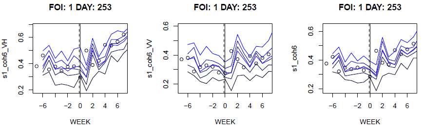
Figure 2. Plots from CreateSignals

What is week0

The analyses consider the difference between week0 and the surrounding weeks. The week0 is the week of the activity observed. The date of activity (week0) is crucial information for the analyses, and inaccuracies will influence the results. In addition the following constraints should be considered:

• First of all, depending on how manifestations have been observed on the ground, there is often some uncertainty about the exact date.

• Second, analyses in this package are done on a weekly basis. The week of the activity will therefore include observations both before and after the activity.

As a result, it is recommended to compare with the week before the activity. The default variables will create 15 week time series where the activity takes place in week 8. If ground observations are collected weakly, the recommendation is to use week0 = 7 in all analyses.

Produce and plot means, standard deviations and t-tests

The first part of the analyses is, for a given activity type, to estimate the means and standard deviations for each of the tested signals, and also to run t.tests to see if the means are significantly different from zero. The analyses are done on a weekly basis. The easiest is to use the functions allSignalMeans and allSignalTTests for these analyses. They are both wrapper functions - around signalMeans and signalTTest. The last two functions have to be called separately for each signal and each activity type, whereas the wrapper functions will keep the different activity types separate, but include all different signals in the analyses. The output from these functions can be used as input in the functions further down. Both of the functions can plot to one or several pdf-documents. They can also open the .pdf-files based on a base name.

The signalMean-function will normally send all plots to two different devices, whereas signalTTest will send the plots to one device. The first of the devices for the signalMean-function will receive confidence plots, if the plotit argument is either "confidence", TRUE or "both". The second device will receive three additional types of plots which might be used for extra analyses.

1. A comparison between mean and median of the signals

2. The median signal value for all the FOIs in the same plot. This plot can become difficult to interpret (many lines) if there are many FOIs.

3. Boxplots of the signal values for all weeks.

As for several of the other functions, it is possible to send subsets of the plots to different devices, by setting the sepPlots argument. allSignalMeans will then need two extra plotting devices for each subset.

# Read all signals and find the names of all signals/indexes
allvar = readSignals(odir)
inds = names(allvar)

# Limit to the first 10 of the default descriptors
stats = SALMS:::bnms[1:10]

# Open two pdfs for plotting the results from the mean function
devs = list()
for (ipdf in 1:2) {pdf(paste0(bdir, "/meanPlot", ipdf, ".pdf")) ; devs[ipdf] = dev.cur()}

# Store all the results from the calculations in evress, which contains an
# array with the means and standard deviations
evress = allSignalMeans(allvar, events = unique(FOIinfo$Event_type), first = FALSE,
                        dels = 0, weighted = FALSE, inds = inds, weeks = 1:15, week0 = 7,
                        weekcorrect = 0, plotit = TRUE, stats = stats,
                        devs = devs, zeroshift = TRUE, FOIinfo = FOIinfo, legend = "before",
                        addNum = FALSE, iprint = 1)
evres = evress$evres
cases = evress$cases
for (ipdf in 1:2) dev.off(devs[ipdf])

# Create three pdfs for t-test output
for (ipdf in 1:3) {pdf(paste0(bdir, "/ttest", ipdf, ".pdf")) ; devs[ipdf] = dev.cur()}

dfs = allSignalTTests(allvar, first = FALSE, dels = 0, weighted = FALSE,
                     inds = inds, dev = devs, weeks = 1:15, stats = stats,
                     week0 = 7, weekcorrect = 0, plotit = TRUE,
                     legend = "before")
# Close the pdfs
for (ipdf in 1:3) dev.off(devs[ipdf])

Figure 3 shows two plots as examples of the output of the signalMeans and signalTTest functions.

The first one shows the mean of the s1_coh6 for all FOIs, with confidence bands based on the standard deviations of the weekly values. The header refers to the activity type (1 in this case), the statistical descriptor and the maximum number of activities used in the plot (the actual number of observations can be lower for some of the weeks).

The second plot shows the means of the NDVI for all FOIs, with the color of the dots according to the confidence level. The lines represent the 95% confidence interval of the mean. The break in the graphs are due to missing values, which can particularly happen for S2-based signals (i.e., from presence of clouds).The header is the same as for the signalMeans.

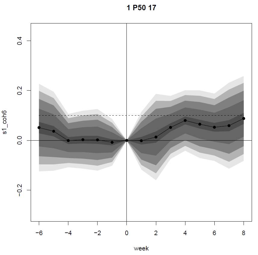
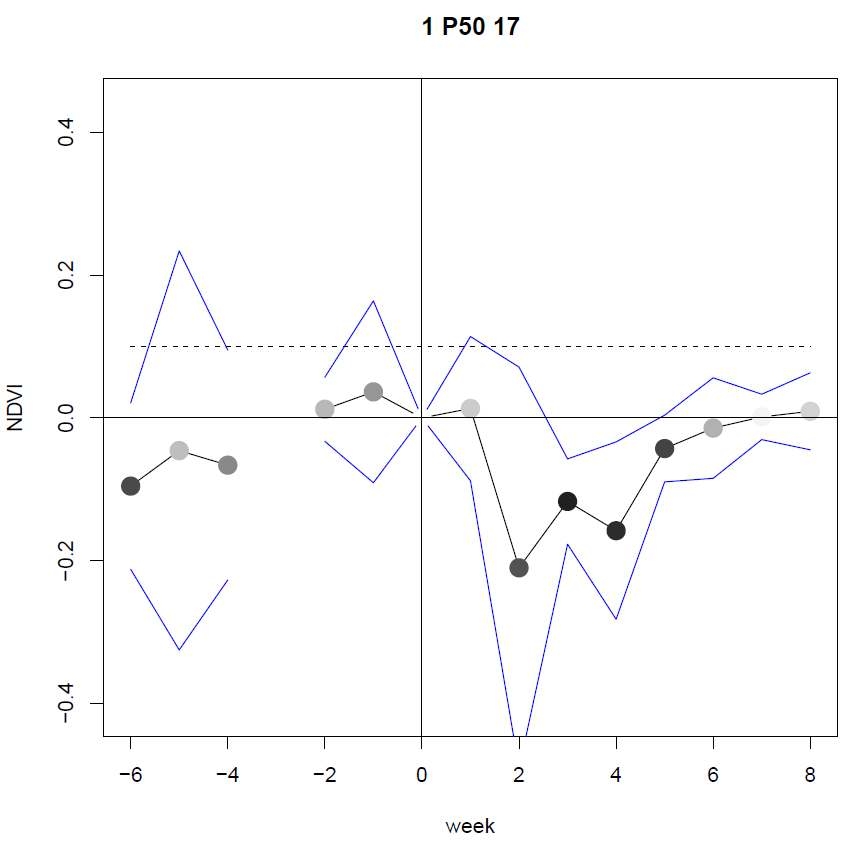
Figure 3. Examples of plots of mean and the t.tests

Analysing signal probabilities

The plots produced by the functions above are useful step-by-step analyses, but too detailed for getting an overview of the capabilities of the different signals/descriptors. The function signalProbability is better for analysing a large set of signals.

First of all, it estimates the probability of the signal being above a threshold. The threshold can either be zero (i.e. the probability that the signal actually increase after an activity), or half the largest change in the weeks following the activity, as a simple threshold which could be used to detect an activity.

When we refer to increases above, the function will internally change the sign of decreasing signals to positive, so that all probabilities will be about being larger than the threshold.

Then it can produce two types of plots, either to the same device, or to two different devices.

The first type of plots are the probability rasters. The first set of these rasters will have the descriptors on the x-axis and the different indexes on the y-axis. The second set will have the weeks on the x-axis, for a particular choice of descriptors.

The probability maps, particularly the first set, give an indication of which signal and which descriptor is the most suitable for the FOIs in the sample. A set of plots are produced. First of all, the plots show different values for p > 0 and p > M, where M is a threshold value that can be used to identify an activity.

For the first set of plots with descriptors on the x-axis, there will be separate plots for each week of the selwks parameter. The week number is the number after “W” in the heading. If there are more than one group of activity types, these are given after “G”. If there is only one activity type, this part of the header is dropped.

The next number is the highest probability in this map. The number after “P” indicates the maximum number of FOIs/activities that have been used for this raster. The last part depends if sortedRasters = TRUE. If yes, the function will also generate a range of plots where the rasters are subsequently ordered according to the values of each individual descriptor/week. Particularly for the descriptors, this gives the opportunity to compare the different descriptors with each other. The sorted rasters can be identified with “S.ind” as a part of the header, followed by the sorting variable.

The second group of plots are graphs with the average value of the change together with the probabilities of the signal increasing. The function will produce four panels on each page. The upper ones show the value and the cumulative value for a particular signal, either as a function of week (only for selected descriptors), or as a function of the descriptor (for selected weeks). The lower panels will show the probability of being above a threshold of zero for the value itself, or for the cumulative sums.

The graphs might be easier to interpret if computeAll = TRUE. This means that the probability values will be estimated for all indexes, not only the ones that the t.test has estimated to have a significant change.

pdf(paste0(bdir, "/sigProb.pdf"))
events = unique(FOIinfo$Event_type)
evres1 = signalProbability(evress$evres, dfs, stats = stats, week0 = 7, weeks = 1:15, selwks = 9:13, selstats = "P50",
                  events = events, inds = inds, cases = cases)
#> [1] "Computing probabilities"
#> [1] " "
#> [1] "plotting raster probabilities"
#> [1] " "
#> [1] "plotting probability graphs"
#> [1] " "
dev.off()
#> png
#>   2

Figure 4 shows an example of a raster probability plot. It shows the maximum probabilities of the signal being above the threshold “M” for each index and statistical descriptor for the selwks period sorted according to the P50 descriptor. Indexes where none of the descriptors show a significant change are not plotted, so in this case this means that B04, s1_bs_rAD and s1_bs_VH_rAD are missing. Sorting the indexes like this, we can see that P50 seems to be good for most indexes for identifying possible activities, although “P25” is better for “BSI” in this particular case.

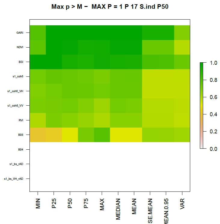
Figure 4. Example of probability raster

Figure 5 shows an example of the graph plots for different statistical descriptors for week 10 for the coherence-based signals. The two panels on the top show the signal change and the cumulative signal change. The two panels on the bottom show the probabilities of the index being above zero for the different descriptors. For this dataset, we can see that the probabilities are highest for the ordinary descriptors, i.e., the mean and the quantiles, except for min and max. Second, we can notice that there is no advantage of using cumulative values (panels to the right) for this data set. This could be different for other data.

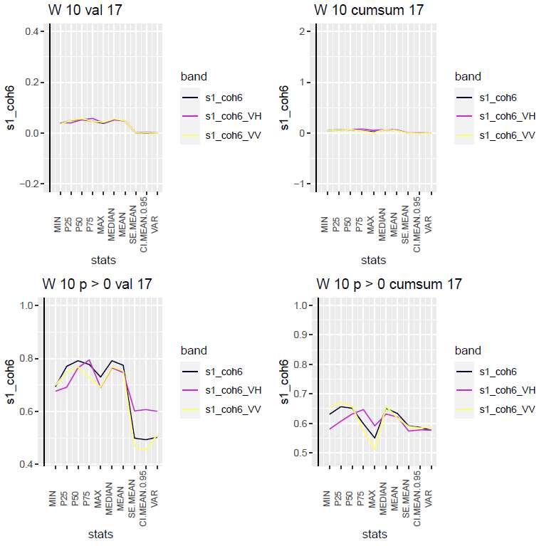
Figure 5. Graphs of signal value change and probabilities for coherence-based signals, both the value itself, and the cumulative sums

Summarizing the results

The functions above let us analyse signals separately. optimalSignal is a function which can help in identifying which descriptor is in general most useful for describing the differences in signal behavior caused by an activity.

It will do this in three different ways, and only for the cases where at least one of the descriptors show a probability above 0.7 of increasing the value after the activity.

1. For how many indexes is a certain descriptor ranked as the first one, for threshold zero or “M”? The weeks are treated separately, so the number can be higher than the number of signals.

2. For how many indexes is a certain descriptor ranked as the last?

3. How good is each descriptor, relatively to the one that is ranked first for a signal? This indicates the relative goodness of a descriptor. Contrary to finding only the first ranked - where two descriptors might be almost similar, but only one included, this gives the relative goodness of each descriptor.

One plot is given for each of the three comparisons, for the two different thresholds.

The output of the function is a data.frame giving the numbers above. Each column with the type describes the three simple classes best (be), worst (bw) and good (bg) descriptors for the different thresholds (0 and T).

pdf(paste0(bdir, "/optimalSignal.pdf"))
dd = optimalSignal(1, inds, evres1, stats)
#> Warning: Removed 4 rows containing missing values (`position_stack()`).
#> Warning: Removed 7 rows containing missing values (`position_stack()`).
#> Warning: Removed 4 rows containing missing values (`position_stack()`).
#> Warning: Removed 6 rows containing missing values (`position_stack()`).
dev.off()
#> png
#>   2

Figure 6 show an example of each of the plots. The left panel shows how “P50” is the most optimal with the highest number of cases where it is ranked as number one. However, it also shows the disadvantage of only counting the highest one, as Median (same as P50) is not the first for any case. The central panel shows that the variance and the confidence interval of the mean are the poorest performing descriptors to be used in this case. The last panel rather looks at the relative goodness of the descriptor. We can here see that there is not a huge difference between the quantiles and the mean although the median is still the most optimal.

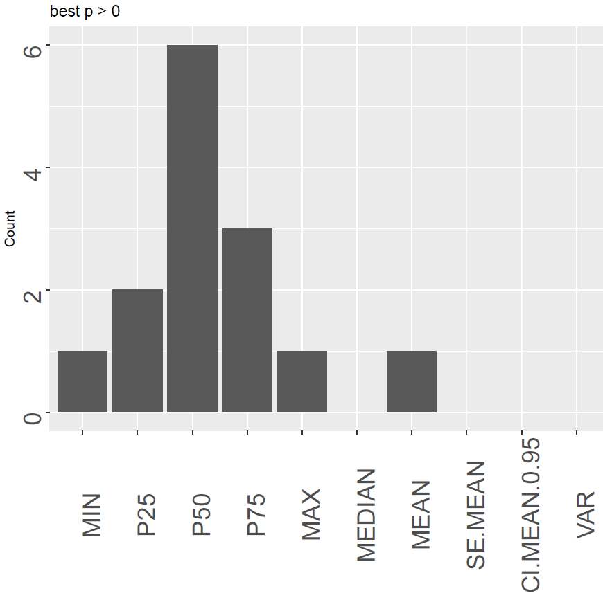
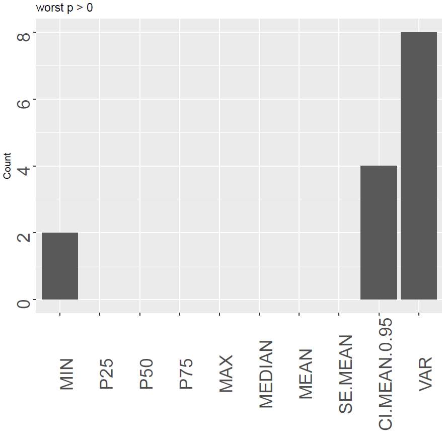
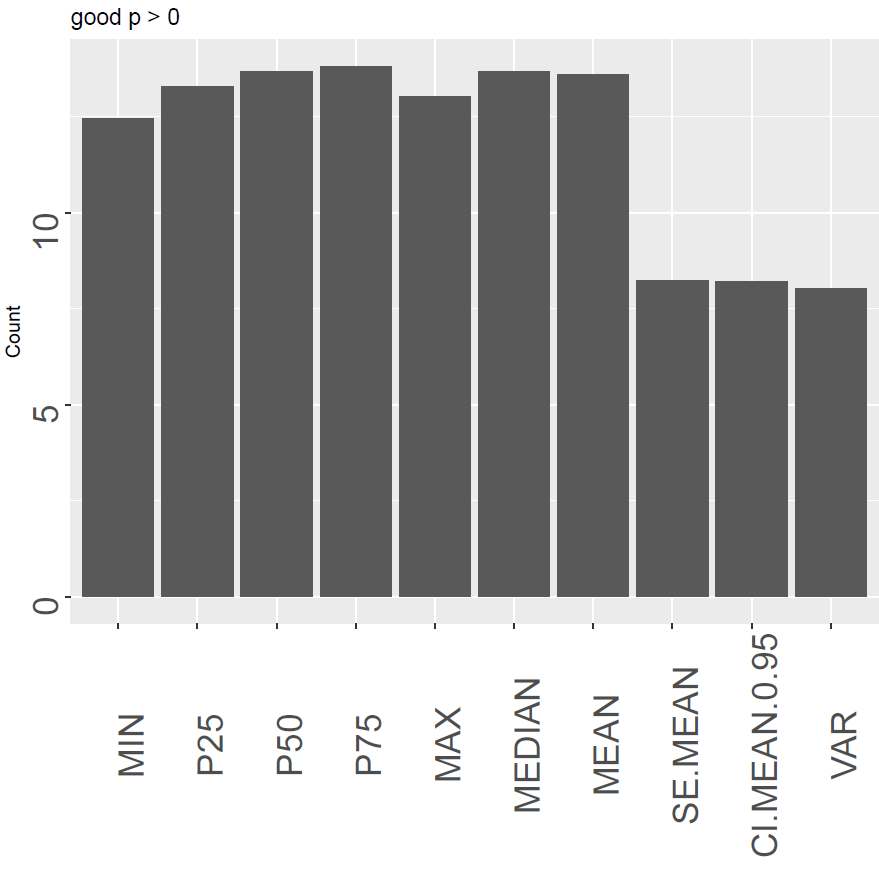
Figure 6. An overview of the best, the poorest and good signal descriptors sums

Correlations

There are many situations where it would be possible to use several signals for detection of a single activity. In this case, it is better to choose signals that are not highly correlated. The function signalCorrelation helps visualizing correlations between the different signals, and will also return a correlation array with the selected descriptors.

pdf(paste0(bdir, "/correlations2.pdf"))
sigCor = signalCorrelations(allvar, stats = c("MIN", "P50"), mar = c(3,3,2,2))
#> [1] "Creating correlation table - activity type 1 indicator: 1"
#> [1] "Creating correlation table - activity type 1 indicator: 2"
#> [1] "Creating correlation table - activity type 1 indicator: 3"
#> [1] "Creating correlation table - activity type 1 indicator: 4"
#> [1] "Creating correlation table - activity type 1 indicator: 5"
#> [1] "Creating correlation table - activity type 1 indicator: 6"
#> [1] "Creating correlation table - activity type 1 indicator: 7"
#> [1] "Creating correlation table - activity type 1 indicator: 8"
#> [1] "Creating correlation table - activity type 1 indicator: 9"
#> [1] "Creating correlation table - activity type 1 indicator: 10"
#> [1] "done correlation  1 1"
dev.off()
#> png
#>   2

Figure 7 shows the correlations between the different signals for the P50descriptor.

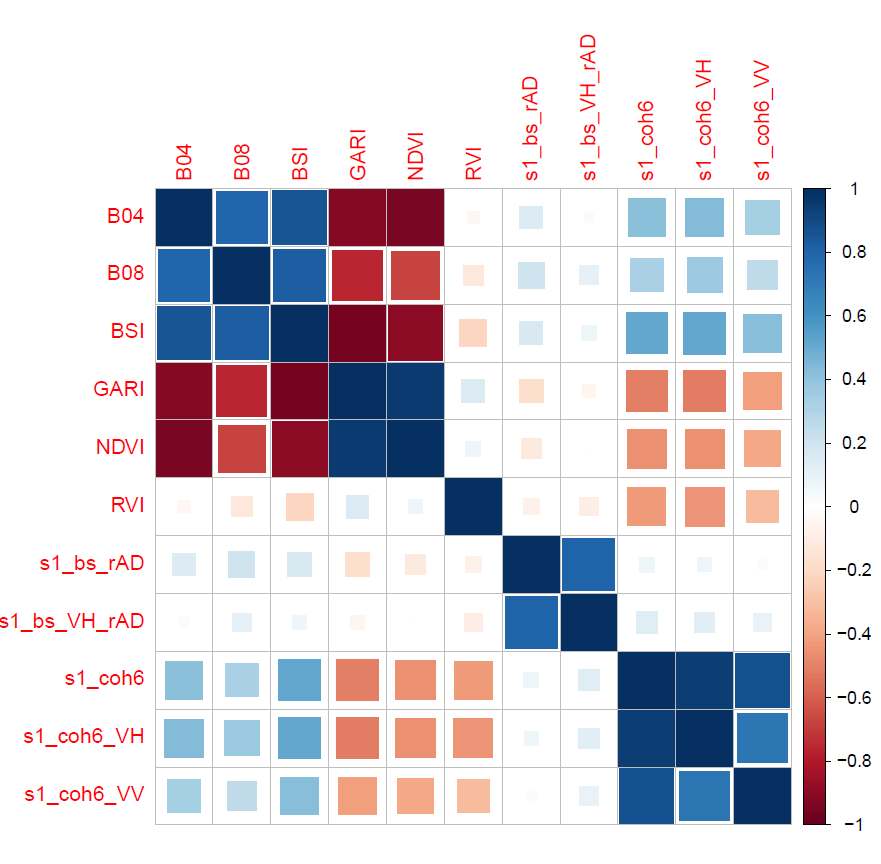
Figure 7. Correlations between signals for the `P50` descriptor

References

Zieliński, Rafal, Jon Olav Skøien, Laura Acquafresca, and Wim Devos. Proposed workflow for optimization of land monitoring systems. JRC130659. Ispra: European Commission. 2022. https://marswiki.jrc.ec.europa.eu/wikicap/images/9/90/JRC130659_final.pdf.