Parcel extraction
Overview
This page describes the use of parcel extraction routines. The general concept of parcel extraction is linked to the marker concept of CAP Check by Monitoring, which assumes that the agricultural parcel is the unit for which we want to confirm the particular agricultural activity.
In computing terms, parcel extraction leads to data reduction: we generate aggregate values from an ensemble of samples by applying some algorithm. The ensemble of samples are the pixels contained within the parcel boundary. The algorithm should, as far as possible, retain the characteristics of the parcel that we are interested in, which is typically the mean, standard deviation and percentiles statistics for the image bands.
The marker principle requires the extraction to run consistently over every CARD image that is available for the period of interest and for all parcels in the region of interest (ROI). Since image cover is usually partial, i.e. only a part of the ROI is covered by a specific image frame (or scene), different combinations of parcel ensembles can be extracted for each individual image.
There are 2 scenarios for parcel extraction: (1) a “burst” scenario, in which all scenes for a significant period (e.g. a year) need to be processed and (2) a “continuous” scenario, in which new scenes are processed incrementally as they arrive on the DIAS. Both scenarios are typically non-interactive, i.e. they should run automatically in the background. Since parcel extractions for distinct scenes are independent processes, they can be easily parallelized. This is particularly important for scenario (1). The typical workload for scenario (2) may not require parallelization.
In the next sections, we first detail the implementation of the parcel extraction routines. We then discuss parallelization using docker swarm (for scenario (1)). Finally, we list some caveats that relate to the use of the extraction routines.
This document assumes familiarity with docker and the database set up used in the JRC-DIAS project.
Implementation details
The high level implementation details of the parcel extraction routines are the following:
The dias_catalogue database table is required to find the metadata for the scenes that cover the ROI, and to keep track of those scenes’ processing status. Other processes may insert new records, e.g. by scanning the DIAS catalogue for newly acquired scenes.
The parcel_set database table is required to get the parcel boundaries and attributes.
As a first step, the oldest scene that intersects the ROI and with status ingested is selected. The status of this scene is changed to inprogress.
The reference attribute for the selected scene is used to compose the key for finding the scene in the S3 store. The scene is downloaded to local disk. Depending on CARD type, more than one object needs to be downloaded (e.g. several bands for S2, the .img and .hdr objects for S1).
All parcel boundaries that are intersecting both the ROI and the footprint of the selected scene are selected from parcel_set.
Using the rasterio and rasterstats python modules, zonal statistics are extracted for each parcel and each band. This is done in chunks of 2000 records.
The extraction results (which include count, mean, stdev, min, max, p25, p50 and p75) are copied into the database table results_table. This table uses foreign keys that reference the unique parcel id in the parcel_set and unique scene id in dias_catalogue.
Upon successful completion of the extraction, the scene status in dias_catalogue is changed to extracted and the local copies of the image file are removed.
Separate versions are kept for each of the ‘bs’, ‘c6’ and ‘s2’ CARD sets, to address the different data formats used. For ‘s2’, the extraction currently handles only the 10m bands B04 (Red) and B08 (NIR) (used for NDVI calculation) and the 20m SCL scene classification band to integrate information on cloud conditions and data quality. This can obviously be reconfigured to include other or more bands. For ‘bs’ and ‘c6’ both VV and VH bands are extracted.
Configuration files
The extraction routines must be configured via 2 parameters files that use the JSON format. In _db_config.json_ the database parameters are defined. This includes the set of connection parameters, the tables used in the relevant queries and the arguments used as query parameters:
{
    "database": {
        "connection": {
            "host": "ip.of.the.dbserver",
            "dbname": "database_name",
            "dbuser": "database_user",
            "dbpasswd": "database_passwd",
            "port": 5432
        },
        "tables": {
            "aoi_table": "tables_with_aois",
            "parcel_table": "table_with_parcels",
            "results_table": "table_with_extracted_signatures"
        },
        "args": {
            "aoi_field": "aoi_name",
            "name": "my_aoi",
            "startdate": "2018-01-01",
            "enddate": "2019-01-01"
        }
    }
}
The aoi_table is a convenience table in which specific ROIs can be defined. It MUST have column name and define its geometry as _wkb_geometry_. This table serves to extract either full national coverages or smaller subsets, e.g. for a province.
parcel_table is assumed to be imported into the database with ogr2ogr and MUST have column names _ogc_fid_ (a unique integer identifier) and _wkb_geometry_. These are normally assigned by ogr2ogr.
It is recommended to name results_table for separate CARD types and the period of extraction. For instance, roi_2018_bs_signatures.
The second parameter file _s3_config.json_ is needed for S3 access, both for the extraction routine and the _download_with_boto3.py_ support script.
{
    "s3": {
        "access_key": "s3_acces_key",
        "secret_key": "s3_secret_key",
        "host": "endpoint_url",
        "bucket": "BUCKET"
    }
}
Run with docker
The extraction code is python3 compatible and requires a number of python modules which are packaged in the glemoine62/dias_py image. A single run can be launched as follows (_working_directory_ is the location of the extraction routine):
cd working_directory
docker run -it --rm -v`pwd`:/usr/src/app glemoine62/dias_py python postgisS2Extract.py
The output will report progress on downloading relevant files, selection of the parcels and zonal statistics extraction. The total number of parcels selected for extraction primarily depends on the location of the image scene. Obviously, this number can range from a few to several 100,000s, and, thus, extraction, can take between 20 and 2000 seconds. The script eliminates parcels for which the extraction results in no data. This can happen in scene boundary areas or fractional scene coverages (common for Sentinel-2).
Parallelization with docker swarm
The extraction routines can easily run in parallel on several VMs with the use of docker swarm. We normally run the configuration as in the figure below:
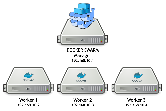
The database is running on the master node and the worker nodes will run one or more extraction tasks. The worker VMs need to have a minimal configuration (a docker installation and the glemoine62/dias_py image), get copies of the relevant extraction routines and configuration files and then join the swarm as workers.
Create VMs
On the DIAS, create 4 new VMs, either through the console, or with the use of the OpenStack command line interface. Minimum configuration should be:
VM of type s3.xlarge.4 (with 4 vCPUs | 16 GB RAM)
Ubuntu 18.04
System disk size of 40 GB (only needed for temporary storage)
No need for external IP. Ensure access from the permanent VM (with external access), using its public key.
Write down the different (internal) IP addresses assigned to the new VMs and enter these in .ssh/config on the permanent VM:
Host vm_new1
  HostName 192.168.*.*
  User cloud
  ServerAliveInterval 10
You can ssh in to each of the new VM instances by using its alias, e.g.:
ssh vm_new1
Install docker and set up docker swarm
On each of the newly created VM, install the minimum configuration, as follows:
ssh vm_new1
sudo apt-get update
sudo apt -y install docker.io
sudo usermod -aG docker $USER
The latter setting avoids the need to run docker commands as sudo and only takes effect after logout/login.
After re-login, get the python3 docker image with the configuration to run the extraction workflow and create a simple directory structure:
ssh vm_new1
docker pull glemoine62/dias_py:latest
mkdir -p dk/data
Copy the required code and configuration files to each of the VMs:
scp postgisS2Extract.py download_with_boto3.py db_config.json s3_config.json vm_new1:/home/eouser/dk
Set up the permanent VM as docker swarm manager:
docker swarm init
This will confirm that the current VM is now the manager and outputs a command line that should be executed on each of the new VMs, to let them join the swarm as “workers”
ssh vm_new1
docker swarm join --token SWMTKN-1-38wcnesfi230xn6p63izm3kr2c4ir6xi4cihvez23grd0phh6u-e0lb90hoq1sm2670yts7vpp1k 192.168.30.116:2377
Check whether all is well:
docker node ls
ID                            HOSTNAME            STATUS              AVAILABILITY        MANAGER STATUS      ENGINE VERSION
7kd7022sf1hzdf9zaqdce86jf *   bastion2            Ready               Active              Leader              18.09.7
z3sghiy1y6kvefaacysgv8cww     project-2019-0001   Ready               Active                                  18.09.7
c7qj1icxfrcqbxas2fq9opm6z     project-2019-0002   Ready               Active                                  18.09.7
tozs74jeexdpiazhc3xqpn7q5     project-2019-0003   Ready               Active                                  18.09.7
fmvmylz2lrfn45upoisz0p7ex     project-2019-0004   Ready               Active                                  18.09.7
i.e. all looks fine.
Configure and run
In order to allow the swarm nodes to communicate with eachother, an overlay network needs to be created:
docker network create -d overlay my-overlay
The docker swarm is configured with the following _docker_compose_s2.yml_ configuration file (assuming S2 extraction):
version: '3.5'
services:
  pg_spat:
    image: mdillon/postgis:latest
    volumes:
      - database:/var/lib/postgresql/data
    networks:
      - overnet
    ports:
      - "5432:5432"
    deploy:
      replicas: 1
      placement:
        constraints: [node.role == manager]

  vector_extractor:
    image: glemoine62/dias_py:latest
    volumes:
      - /home/eouser/es:/usr/src/app
    networks:
      - overnet
    depends_on:
      - pg_spat
    deploy:
      replicas: 8
      placement:
        constraints: [node.role == worker]
    command: python postgisS2Extract.py

networks:
  overnet:
volumes:
  database:
This will create one task, _pg_spat_, on the manager node (i.e. the permanent VM), that runs the database server, using the mounted volume where the database outputs are written. The _vector_extractor_ task is started on the worker nodes, as 8 replicas (thus 2 tasks on each node).
The swarm can be started as follows:
docker stack deploy -c docker_compose_s2.yml s2swarm
The swarm runs a stack of services in the background, for which the status can be checked with:
docker service ls
or the service logs displayed with:
docker service logs -f s2swarm_vector_extractor
Note that the stack continues to launch new processes. After some time there are no longer ingested candidate images left in the dias_catalogue. Check the logs to ensure that all processes return with the message “No image with status ‘ingested’ found”. Stop the stack with the command:
docker stack rm s2swarm
Caveats
The extraction routines assume standard naming of a number of required columns in the various data base table (see above). Errors will be thrown if this is not applied consistently.
The extraction routines use the copy statement to write to the results_table signatures data base, because this is much faster than insert statements. The results_table should preferable NOT have indices defined on the foreign key columns, as this will slow down mass copying into the table.
Docker stack continues to run even if no data available to process.