POST requests

Taking the next step: Using POST with RESTful services to get tailor made selections

Please read up on the generic characteristics of the RESTful service AND RESTful queries for chip selections BEFORE using the query described here.

rawChipsBatch

This query extends rawChipByLocation by providing a faster parallel extraction.

It requires the POST method, instead of the GET methods used in the previous pages, because the parameters are now lists of detailed references to individual chip selections. This also means that the query no longer works in a standard browser (unless you install special extensions like postman in your browser, though that is mostly useful as a debug tool).

Using POST has the additional advantage that it is much easier to provide request parameters as more complex structures, e.g. including lists. We will post JSON dictionary structures.

The overall idea behind using rawChipBatch is that you already have made a selection of specific items that you want to collect from the server. The items are passed as a list, which is then extracted on parallel VMs on the server. A common scenario for Sentinel-2 selection would be to first screen the SCL information for a parcel (either using parcelTimeSeries or rawChipByLocation) and then POST the cloud-free selections to retrieve the bands of interest.

The cartesian product of selected references and unique bands is returned (e.g. if 4 references and 3 bands are provided as parameters, 12 GeoTIFF chips are produced).

Currently, parameter values can be as follows:

Parameters	Format	Description
lon, lat	float numbers	Any geographical coordinate where Level-2A Sentinel-2 is available
tiles	list of strings	Time window for which Level-2A Sentinel-2 is available (after 27 March 2018)
bands	list of strings	Sentinel-2 band name. Selection out of [‘B02’, ‘B03’, ‘B04’, ‘B08’] (10 m bands) or [‘B05’, ‘B06’, ‘B07’, ‘B8A’, ‘B11’, ‘B12’, ‘SCL’] (20 m bands).
chipsize	int	1280 (default), truncated to 5120, if larger

returns

A JSON dictionary with date labels and relative URLs to cached GeoTIFFs.

You need a client script to transfer the GeoTIFFs and run analysis on it.

Example test script

Based on the result of the example script for rawChipByLocation the following script retrieves the bands B04, B08 and B11 for the 3 scenes for which the parcel histogram showed that they are without cloud masked SCL pixels. Instead of downloading the bands from cache, we generate NDVI directly from the cached bands B08 and B04, and scale the result to a byte image which will be given a matplotlib color map of choice.

For the simple client side image processing tasks, you need:

Simple client-side image processing

Get the code

import requests

import imgLib

username = 'YOURUSERNAME'
password = 'YOURPASSWORD'
host = '0.0.0.0'

# Authenticate directly in URL
tifUrlBase = f"http://{username}:{password}@{host}"
url = tifUrlBase + "/query/rawChipsBatch"

payloadDict = {
  "lon": 5.66425,
  "lat": 52.69444,
  "tiles": ["S2B_MSIL2A_20190617T104029_N0212_R008_T31UFU_20190617T131553",
            "S2A_MSIL2A_20190625T105031_N0212_R051_T31UFU_20190625T134744",
            "S2B_MSIL2A_20190620T105039_N0212_R051_T31UFU_20190620T140845"],
  "bands": ["B08", "B04", "B11"],
  "chipsize": 2560
}

response = requests.post(url, json=payloadDict)

jsonOut = response.json()

# Instead of transfering the image bands from cache
# generate an normalizedDifference output directly from the cache URLs
for c in jsonOut.get('chips'):
    if c.endswith('B08.tif'):
        name = c.split('/')[-1].replace('B08', 'NDVI')
        url0 = tifUrlBase + c
        url1 = url0.replace('B08.tif', 'B04.tif')

        imgLib.normalizedDifference(url0, url1, name)
        imgLib.scaled_palette(name, 0, 1, 'RdYlGn')

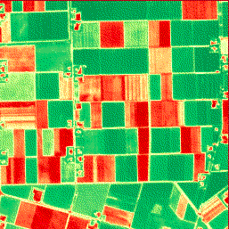
The scaled NDVI output of 2019-06-25 rendered as a PNG.

Home work: derive the NDVI histogram for parcel at this location and create a plot with the color map of the scaled version.

rawS1ChipsBatch

In analogue to the rawChipBatch query, this query retrieves Sentinel-1 chips. Since Sentinel-1 chips never have cloud issues, we don’t need to cloud check first and make a specific selection. Instead, we can fall back to a date range selection. However, we prefer the convenience of POSTing JSON structures to pass on the request parameters. We further simplify by always returning both polarization (VV and VH for IW image mode over land).

WARNING

There are generally more Sentinel-1 observations then Sentinel-2 observations, where both ascending and descending orbits are acquired (e.g. most of Europe). Thus, the chip limit is generally reached with shorted time windows. Caching rules apply as usual.

Sentinel-1 chips are ONLY available where the imagery is processed to CARD (Copernicus Analysis Ready Data). This is only the case for selected European areas (on CREODIAS).

Sentinel-1 chips are selected from larger image sets and are always generated as float32 images. This (currently) takes more time than for Sentinel-2 and leads to larger file size (e.g. for transfer).

Request parameters are as follows:

Currently, parameter values can be as follows:

Parameters	Format	Description
lon, lat	float numbers	Any geographical coordinate where Level-2A Sentinel-2 is available
dates	list of strings	Start and end date of selection time window formatted as YYYY-mm-dd
chipsize	int	1280 (default), truncated to 5120, if larger
plevel	string	‘CARD-BS’ for geocoded GRD backscattering coefficient, or ‘CARD-COH6’ for 6-day coherence

returns

A JSON dictionary with date labels and relative URLs to cached GeoTIFFs.

In the client code script below, we grab the GeoTIFFs for the Sentinel-1 CARD-BS and CARD-COH6 sets for the same area as above. We then compose some of that data into a false colour composite of mean VV and VH backscattering coeffients and the 6-day coherence for the period 2019-06-14 to 2019-06-20. The composite is byte-scaled for display purposes.

Get the code

import requests

import rasterio
import numpy as np

# Should move to imgLib later
def byteScale(img, min, max):
    return np.clip(255 * (img - min) /(max - min), 0, 255).astype(np.uint8)

username = 'YOURUSERNAME'
password = 'YOURPASSWORD'
host = '0.0.0.0'

tifUrlBase = f"http://{username}:{password}@{host}"
url = tifUrlBase + "/query/rawS1ChipsBatch"
payloadDict = {
  "lon": 5.66425,
  "lat": 52.69444,
  "dates": ["2019-06-10", "2019-06-25"],
  "chipsize": 2560,
  "plevel": 'CARD-BS'
}

# First get the CARD-BS
response = requests.post(url, json=payloadDict)
json_BS = response.json()

# then get CARD-COH6
payloadDict['plevel'] = 'CARD-COH6'
response = requests.post(url, json=payloadDict)
json_C6 = response.json()

# Now let's do some arty compositing
# We'll generate a mean VV and VH for the period
# and add coherence

g0 = [f for f in json_BS.get('chips') if f.find('20190614')!=-1]
g1 = [f for f in json_BS.get('chips') if f.find('20190620')!=-1]
c0 = [f for f in json_C6.get('chips') if f.find('20190614')!=-1 and f.find('20190620')!=-1]

g0VV = [g for g in g0 if g.find('VV')!=-1][0]
g0VH = g0VV.replace('VV', 'VH')
g1VV = [g for g in g1 if g.find('VV')!=-1][0]
g1VH = g1VV.replace('VV', 'VH')

# We only open the VV coherence band
c0VV = [c for c in c0 if c.find('VV')!=-1][0]

with rasterio.open(tifUrlBase + g0VV) as src:
    vv = src.read(1)
    kwargs = src.meta.copy()

# Take the average of the 2 VV bands and convert to dB
with rasterio.open(tifUrlBase + g1VV) as src:
    vv = 10.0*np.log10((vv + src.read(1))/2)

with rasterio.open(tifUrlBase + g0VH) as src:
    vh = src.read(1)

with rasterio.open(tifUrlBase + g1VH) as src:
    vh = 10.0*np.log10((vh + src.read(1))/2)

with rasterio.open(tifUrlBase + c0VV) as src:
    c6 = src.read(1)

kwargs.update({'count': 3, 'dtype': np.uint8})
with rasterio.open(f"test.tif", 'w',**kwargs) as sink:
    sink.write(byteScale(vv, -15.0, -3.0),1) # R
    sink.write(byteScale(vh, -20.0, -8.0),2) # R
    sink.write(byteScale(c6, 0.2, 0.9),3) # R

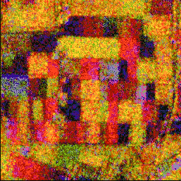
The result is compared to the NDVI image of 2019-06-25.

At first sight, you will notice the speckly appearance of the S1 composite versus the crisp Sentinel-2 NDVI, which even shows fine inner-parcel details. But look closer, and you find more variation in the S1 composite. You can easily separate winter cereals from broadleaf crops, for instance, something that is nearly impossible in the S2 NDVI. Sparsely vegetated fields show some coherence (blue tints), etc.