Parcel Time Series

parcelTimeSeries

Using RESTful services to get parcel time series

Extract time series statistics from the Sentinel data are available, both actual and archived, for all parcels in an annual declaration set.

The table below shows the parameters for time series selection.

Parameters	Description	Values	Default value
aoi	Area of Interest (Member state or region code)	e.g.: at, pt, ie, etc.
year	year of parcels dataset	e.g.: 2018, 2019
pid	parcel ID
ptype	parcels type	b, g, m, atc.
tstype	Sentinel-2 Level 2A, S1 CARD Backscattering Coefficients, S1 CARD 6-day Coherence	s2, bs, c6, scl	s2
scl	Include scl in the s2 extraction, for use in cloud screening	True or False	True
ref	Include Sentinel image reference in time series	True or False	False
tsformat	parcels type	csv, json	json

Examples: Change the parameters aoi, year and pid based on your provided parcels data.

Example 1, returns the S2 time series of the parcel with SCL histograms and image reference, https://cap.users.creodias.eu/query/parcelTimeSeries?aoi=ms&year=2020&pid=123&tstype=s2&scl=True&ref=True
Example 2, returns the S1 Backscattering Coefficients time series of the parcel, https://cap.users.creodias.eu/query/parcelTimeSeries?aoi=ms&year=2020&pid=123&tstype=bs
Example 3, returns the S1 6-day Coherence time series of the parcel, https://cap.users.creodias.eu/query/parcelTimeSeries?aoi=ms&year=2020&pid=123&tstype=c6
Example 4, returns only the SCL histogram for the selected parcel, https://cap.users.creodias.eu/query/parcelTimeSeries?aoi=ms&year=2020&pid=123&tstype=scl

returns

Key	Values	Description
date_part	a list of timestamps	as seconds since ‘Unix epoch’ (1970-01-01 00:00:00 UTC)
band	a list of image bands	Missing if band query parameter is provided
count	a list of counts	count of pixels extracted for each parcel and observation
mean	a list of means	mean etc.
std	a list of stds	standard deviation etc.
min	a list of mins	min etc.
max	a list of maxs	max etc.
p25	a list of p25s	25% histogram percentile etc.
p50	a list of p50s	50% histogram percentile etc.
p75	a list of p75s	75% histogram percentile etc.

weatherTimeSeries

Example: Change the parameters aoi, year and pid based on your provided parcels data.

Example 1, returns the weather time series of the parcel, https://cap.users.creodias.eu/query/weatherTimeSeries?aoi=ms&year=2020&pid=123

returns

Key	Description
meteo_date	a list of timestamps as seconds since ‘Unix epoch’ (1970-01-01 00:00:00 UTC)
tmean	a list of means
tmin	a list of mins
tmax	a list of maxs
prec	precipitation

Simple python client to plot parcel Time Series

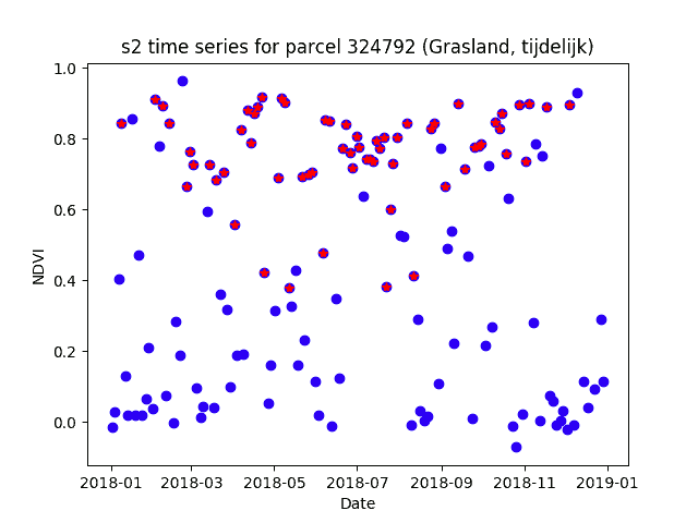
We show a complete example on how to use the RESTful queries in a python script. The script first requests the parcel details at the geographical location, and than retrieves the Sentinel-2 time series in a second request. The response of the latter query is parsed into a pandas DataFrame, which allows some data reorganisation and cleanup. The cleaned data is used to generate an NDVI profile which is then plotted, resulting in a figure as the one below. The blue dots are showing all NDVI values, those with a red inset are for observations that are cloud-free according to the “scene classifier” band of Sentinel 2 Level 2A.

Get the source

"""
NDVI plot example
"""

import json
import requests
import pandas as pd
import matplotlib.pyplot as plt
import matplotlib.dates as mdates
from datetime import timedelta


# Define your credentials here
username = 'YOURUSERNAME'
password = 'YOURPASSWORD'
host = 'http://0.0.0.0'

# Set parcel query parameters
aoi = 'ms'
year = '2020'
ptype = ''
lon = '5.1234'
lat = '50.1234'

# Set the cloud Scene Classification (SC) values.
scl = '3_8_9_10_11'


# ------ Plot NDVI
tstype = 's2'

# Get parcel information for a given location
parcelurl = """{}/query/parcelByLocation?aoi={}&year={}&lon={}&lat={}&withGeometry=True&ptype={}"""
response = requests.get(parcelurl.format(
    host, aoi, year, lon, lat, ptype), auth=(username, password))
parcel = json.loads(response.content)

pid = parcel['pid'][0]
crop_name = parcel['cropname'][0]
area = parcel['area'][0]

# Get the parcel Time Series
tsurl = """{}/query/parcelTimeSeries?aoi={}&year={}&pid={}&tstype={}&ptype={}"""
response = requests.get(tsurl.format(
    host, aoi, year, pid, tstype, ptype), auth=(username, password))
# Directly create a pandas DataFrame from the json response
# This should work even if the response is and empty dictionary
df = pd.read_json(response.content)

df['date'] = pd.to_datetime(df['date_part'], unit='s')
start_date = df.iloc[0]['date'].date()
end_date = df.iloc[-1]['date'].date()
print(f"From '{start_date}' to '{end_date}'.")

pd.set_option('max_colwidth', 200)
pd.set_option('display.max_columns', 20)

# Plot settings are confirm IJRS graphics instructions
plt.rcParams['axes.titlesize'] = 16
plt.rcParams['axes.labelsize'] = 14
plt.rcParams['xtick.labelsize'] = 12
plt.rcParams['ytick.labelsize'] = 12
plt.rcParams['legend.fontsize'] = 14

df.set_index(['date'], inplace=True)

dfB4 = df[df.band.isin(['B4', 'B04'])].copy()
dfB8 = df[df.band.isin(['B8', 'B08'])].copy()
datesFmt = mdates.DateFormatter('%-d %b %Y')

# Plot Cloud free NDVI.
dfNDVI = (dfB8['mean'] - dfB4['mean']) / (dfB8['mean'] + dfB4['mean'])

df['cf'] = pd.Series(dtype='str')
scls = scl.split('_')
for index, row in df.iterrows():
    if any(x in scls for x in [*row['hist']]):
        df.at[index, 'cf'] = 'False'
    else:
        df.at[index, 'cf'] = 'True'
cloudfree = (df['cf'] == 'True')
cloudfree = cloudfree[~cloudfree.index.duplicated()]

fig = plt.figure(figsize=(16.0, 10.0))
axb = fig.add_subplot(1, 1, 1)

axb.set_title(f"Parcel {pid} (crop: {crop_name}, area: {area:.2f} sqm)")

axb.set_xlabel("Date")
axb.xaxis.set_major_formatter(datesFmt)

axb.set_ylabel(r'NDVI')
axb.plot(dfNDVI.index, dfNDVI, linestyle=' ', marker='s',
         markersize=10, color='DarkBlue',
         fillstyle='none', label='NDVI')

axb.plot(dfNDVI[cloudfree].index, dfNDVI[cloudfree],
         linestyle=' ', marker='P',
         markersize=10, color='Red',
         fillstyle='none', label='Cloud free NDVI')


axb.set_xlim(start_date, end_date + timedelta(1))
axb.set_ylim(0, 1.0)

axb.legend(frameon=False)

plt.show()