Sentinel image chips
Using RESTful services to get parcel time series as image chips
Please read up on the generic characteristics of the RESTful service before using the queries described here.
WARNING: The query described here is resource intensive. It starts a complex task that involves communication between docker containers and parallel execution on several DIAS VMs. The following limitations apply:
Chip extraction is for Level-1C (L1C) and Level-2A (L2A) Sentinel-2. L2A is not available everywhere, but generally in the CbM onboarding Member States and those in other pilots (e.g. SEN4CAP, EOSC-EAP) where CREODIAS was used. L1C is available globally.
Selection is by date range. The current limit per request is 24 chips. No cloud filtering is applied. Shorten the time window if it leads to > 24 chips being selected (error output is still rudimentary).
The service applies a simple rule to exclude duplicate chips for the same date (e.g. in tile overlaps). However, a location may be in a multiple orbit overlap, which will generate denser time series than the usual 5 day repeat cycle of the A and B sensors. Thus, you may need to shorten the time window in order not to exceed the 24 chip limit.
The server has a simple caching mechanism. If you run the query again, for the same location, with a different time window, it will only generate the new chips and return the rest from cache. This can be used to create longer time series faster. In case you do not want the cashed chips, you can request only the new chips by changing slightly the location.
The cache is flushed regularly, typically at midnight (CET).
Do not refresh the link if it is still running, as it will start a new selection process and currently screws up the sequence.
NOTE: The use of these RESTful queries on JRC RESTful example is meant for occassional use and testing. If you have a use case that requires many chip generations, please contact us for alternative methods.
All requests are logged, using your internet address (IP). Furthermore, the caching is based on a combination of your IP and query parameters. We regularly check the cache and will contact you in case we detect excessive use.
chipByLocation
Generates a series of extracted Sentinel-2 LEVEL2A segments of 128x128 pixels as a composite of 3 bands.
Currently, parameter values can be as follows:
Parameters |
Format |
Description |
|---|---|---|
lon, lat |
a string representing a float number |
Any geographical coordinate where Level-2A Sentinel-2 is available |
start_date, end_date |
YYYY-mm-dd |
Time window for which Level-2A Sentinel-2 is available (after 27 March 2018) |
lut |
Low_High |
A pair of float values between 0 and 100 separated by an underscore (_). Low must be smaller than High. Defaults to 5_95 |
lut |
LB1_HB1_LB2_HB2_LB3_HB3 |
3 pairs of float values, with each value separated by an underscore (_). Each pair are the absolute low and high thresholds, applied to the band selection |
bands |
Bn1_Bn2_Bn3 |
3 Sentinel-2 band names. One of [‘B02’, ‘B03’, ‘B04’, ‘B08’] (10 m bands) or [‘B05’, ‘B06’, ‘B07’, ‘B8A’, ‘B11’, ‘B12’] (20 m bands). 10m and 20m bands can be combined. The first band determines the resolution in the output composite. Defaults to B08_B04_B03. |
plevel |
string |
LEVEL2A, LEVEL1C. Use LEVEL1C where LEVEL2A is not avaiable |
returns
An HTML page that displays the selected chips in a table with max. 8 columns.
rawChipByLocation
rawChipByLocation - rawChipByParcelID
Generates a series of extracted Sentinel-2 LEVEL2A segments of 128x128 (10m resolution bands) or 64x64 (20 m) pixels as list of full resolution GeoTIFFs.
Table: rawChipByLocation Parameters
Parameters |
Description |
Values |
Default Value |
|---|---|---|---|
lon |
longitude in decimal degrees |
e.g.: 6.31 |
|
lat |
latitude in decimal degrees |
e.g.: 52.34 |
|
start_date, end_date |
Time window for which Level-2A Sentinel-2 is available (after 27 March 2018) |
Format: YYYY-mm-dd |
|
band |
Sentinel-2 band name. One of [‘B02’, ‘B03’, ‘B04’, ‘B08’] (10 m bands) or [‘B05’, ‘B06’, ‘B07’, ‘B8A’, ‘B11’, ‘B12’, ‘SCL’] (20 m bands). |
Format: BXX |
|
chipsize |
size of the chip in pixels |
< 5120 |
1280 |
plevel |
Processing levels. Use LEVEL1C where LEVEL2A is not avaiable |
LEVEL2A, LEVEL1C |
LEVEL2A |
Table: rawChipByParcelID Parameters
Parameters |
Description |
Example call |
Values |
|---|---|---|---|
aoi |
Area of Interest (Member state or region code) |
e.g.: at, pt, ie, etc. |
|
year |
year of parcels dataset |
e.g.: 2018, 2019 |
|
pid |
parcel id |
||
ptype |
parcels type |
b, g, m, atc. |
|
start_date, end_date |
Time window for which Level-2A Sentinel-2 is available (after 27 March 2018) |
Format: YYYY-mm-dd |
|
band |
Sentinel-2 band name. One of [‘B02’, ‘B03’, ‘B04’, ‘B08’] (10 m bands) or [‘B05’, ‘B06’, ‘B07’, ‘B8A’, ‘B11’, ‘B12’, ‘SCL’] (20 m bands). |
Format: BXX |
|
chipsize |
size of the chip in pixels |
< 5120 |
1280 |
plevel |
Processing levels. Use LEVEL1C where LEVEL2A is not avaiable |
LEVEL2A, LEVEL1C |
LEVEL2A |
Examples:
Example 1: List of downloadable Sentinel images for a given location: https://cap.users.creodias.eu/query/rawChipByLocation?lon=5.123&lat=55.123&start_date=2020-01-01&end_date=2020-01-30&band=SCL&chipsize=920
Example 2: List of downloadable Sentinel images for a given parcel ID: https://cap.users.creodias.eu/query/rawChipByParcelID?aoi=MS&year=2020&pid=1234&start_date=2020-01-01&end_date=2020-01-30&band=B04&chipsize=920
returns
A JSON dictionary with date labels and relative URLs to cached GeoTIFFs e.g.:
{"dates": ["20200101T105441", "..."], "chips": ["/dump/..._20200101T121106.SCL.tif", "..."]}
You will need to add the host to download the image e.g.:
https://cap.users.creodias.eu/dump/..._20200129T130207.SCL.tif
The preferred way is to use a client script to transfer the GeoTIFFs and run analysis on it.
Example client code.
The code example builds on the client code of the basic RESTful services, and integrates some more advanced processing concepts that help build up to more advanced logic in the next steps.
First, we locate a parcel by location, as before, but now use the geometry that is (optionally) returned by parcelByLocation to refine the positioning of the chip selection. This introduces some basic feature geometry handling that is possible with the GDAL python libraries, including geometry creation for JSON, reprojection and centroid extraction. For the centroid position, the rawChipByLocation is launched to retrieve the SCL band for the Sentinel-2 Level-2A data. SCL is produced in the atmospheric correction step of SEN2COR, and contains mask values that link to the Scene CLassification. These mask values are useful to determine whether a pixel (in the parcel) is cloud free.
rawChipByLocation first stages the selections, as GeoTIFFs, in the user cache on the server and then returns a JSON dictionary with the file locations. This information is then used to download the GeoTIFFs to local disk. Finally, we iterate through the list of downloaded GeoTIFFs and extract the histogram for the parcel pixels.
import sys
import glob
import json
import requests
import rasterio
import pandas as pd
from datetime import datetime
from rasterstats import zonal_stats
from osgeo import osr, ogr

# Define your credentials here
username = 'YOURUSERNAME'
password = 'YOURPASSWORD'
host = 'http://0.0.0.0'

# Set parcel query parameters
aoi = 'ms'
year = '2020'
ptype = ''
lon = '5.1234'
lat = '50.1234'


# Parse the response with the standard json module
# Get parcel information for a given location
parcelurl = """{}/query/parcelByLocation?aoi={}&year={}&lon={}&lat={}&withGeometry=True&ptype={}"""
response = requests.get(parcelurl.format(host, aoi, year, lon, lat, ptype), auth = (username, password))
parcel = json.loads(response.content)

# Check response
if not parcel:
    print("Parcel query returned empty result")
    sys.exit()
elif not parcel.get(list(parcel.keys())[0]):
    print(f"No parcel found in {parcels} at location ({lon}, {lat})")
    sys.exit()

print(parcelurl.format(host, aoi, year, lon, lat, ptype))

# Create a valid geometry from the returned JSON withGeometry
geom = ogr.CreateGeometryFromJson(parcel.get('geom')[0])

source = osr.SpatialReference()
source.ImportFromEPSG(parcel.get('srid')[0])

# Assign this projection to the geometry
geom.AssignSpatialReference(source)

target = osr.SpatialReference()
target.ImportFromEPSG(4326)

transform = osr.CoordinateTransformation(source, target)

# And get the lon, lat for its centroid, so that we can center the chips on
# the parcel
centroid = geom.Centroid()
centroid.Transform(transform)

# Use pid for next request
pid = parcel['pid'][0]
cropname = parcel['cropname'][0]

# Set up the rawChip request
rawurl = """{}/query/rawChipByLocation?lon={}&lat={}&start_date={}&end_date={}&band={}&chipsize={}"""

# Images query parameter values
start_date='2019-06-01'
end_date ='2019-06-30'
band = 'SCL'    # Start with the SCL scene, to check cloud cover conditions
chipsize = 2560 # Size of the extracted chip in meters (5120 is maximum)

print(rawurl.format(host, str(centroid.GetY()), str(centroid.GetX()), start_date, end_date, band, chipsize))
response = requests.get(rawurl.format(host, str(centroid.GetY()), str(centroid.GetX()), start_date, end_date, band, chipsize), auth = (username, password))

# Directly create a pandas DataFrame from the json response
df = pd.read_json(response.content)

# Check for an empty dataframe
if df.empty:
    print(f"rawChip query returned empty result")
    sys.exit()

print(df)

# Download the GeoTIFFs that were just created in the user cache
for c in df.chips:
    url = f"{host}{c}"
    res = requests.get(url, stream=True)
    outf = c.split('/')[-1]
    print(f"Downloading {outf}")
    handle = open(outf, "wb")
    for chunk in res.iter_content(chunk_size=512):
        if chunk:  # filter out keep-alive new chunks
            handle.write(chunk)
    handle.close()

# Check whether our parcel is cloud free

# We should have a list of GeoTIFFs ending with .SCL.tif
tiflist = glob.glob('*.SCL.tif')

for t in tiflist:
    with rasterio.open(t) as src:
        affine = src.transform
        CRS = src.crs
        data = src.read(1)

    # Reproject the parcel geometry in the image crs
    imageCRS = int(str(CRS).split(':')[-1])

    # Cross check with the projection of the geometry
    # This needs to be done for each image, because the parcel could be in a
    # straddle between (UTM) zones
    geomCRS = int(geom.GetSpatialReference().GetAuthorityCode(None))

    if geomCRS != imageCRS:
        target = osr.SpatialReference()
        target.ImportFromEPSG(imageCRS)
        source = osr.SpatialReference()
        source.ImportFromEPSG(geomCRS)
        transform = osr.CoordinateTransformation(source, target)
        geom.Transform(transform)

    # Format as a feature collection (with only 1 feature) and extract the histogram
    features = { "type": "FeatureCollection",
        "features": [{"type": "feature", "geometry": json.loads(geom.ExportToJson()), "properties": {"pid": pid}}]}
    zs = zonal_stats(features, data, affine=affine, prefix="", nodata=0, categorical=True, geojson_out=True)

    # This has only one record
    properties = zs[0].get('properties')

    # pid was used as a dummy key to make sure the histogram values are in 'properties'
    del properties['pid']

    histogram = {int(float(k)):v for k, v in properties.items()}
    print(t, histogram)
The code creates the following output:
S2A_MSIL2A_20190615T105031_N0212_R051_T31UFU_20190615T121337.SCL.tif {9: 187}
S2A_MSIL2A_20190602T104031_N0212_R008_T31UFU_20190602T140340.SCL.tif {8: 187}
S2A_MSIL2A_20190605T105031_N0212_R051_T31UFU_20190605T152839.SCL.tif {9: 187}
S2B_MSIL2A_20190617T104029_N0212_R008_T31UFU_20190617T131553.SCL.tif {4: 187}
S2B_MSIL2A_20190607T104029_N0212_R008_T31UFU_20190607T135245.SCL.tif {8: 187}
S2A_MSIL2A_20190622T104031_N0212_R008_T31UFU_20190622T120726.SCL.tif {4: 1, 5: 44, 7: 42, 8: 63, 9: 37}
S2B_MSIL2A_20190610T105039_N0212_R051_T31UFU_20190610T133632.SCL.tif {8: 26, 10: 161}
S2A_MSIL2A_20190612T104031_N0212_R008_T31UFU_20190612T133140.SCL.tif {8: 187}
S2A_MSIL2A_20190625T105031_N0212_R051_T31UFU_20190625T134744.SCL.tif {4: 186, 5: 1}
S2B_MSIL2A_20190627T104029_N0212_R008_T31UFU_20190627T135004.SCL.tif {9: 187}
S2B_MSIL2A_20190620T105039_N0212_R051_T31UFU_20190620T140845.SCL.tif {4: 187}
i.e., for each image set, the histogram (a dictionary) shows how many of the 187 pixels included in the parcel (at 20 m resolution) are in each SCL class. The SCL class keys have the following meaning:
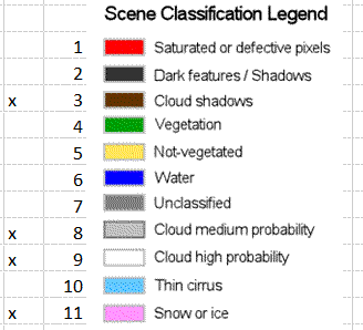
(Courtesy of Csaba Wirnhardt, JRC)
thus, only 3 out of the 11 image in June 2018 are cloud free. One has mixed values, and 7 are completely cloud covered.
You can now decide to go pick up the relevant bands for the 4 cloud free acquisitions. This can, in principle, be done with rawChipByLocation but that is not a very efficient procedure, because that query does not benefit well from parallel processing.
Continue on the next WIKI page to find a more advanced solution.